Metric and KPI Identification
Collaborated with UNICEF information specialist to define and implement critical metrics and KPIs, ensuring the dashboard meets user needs.

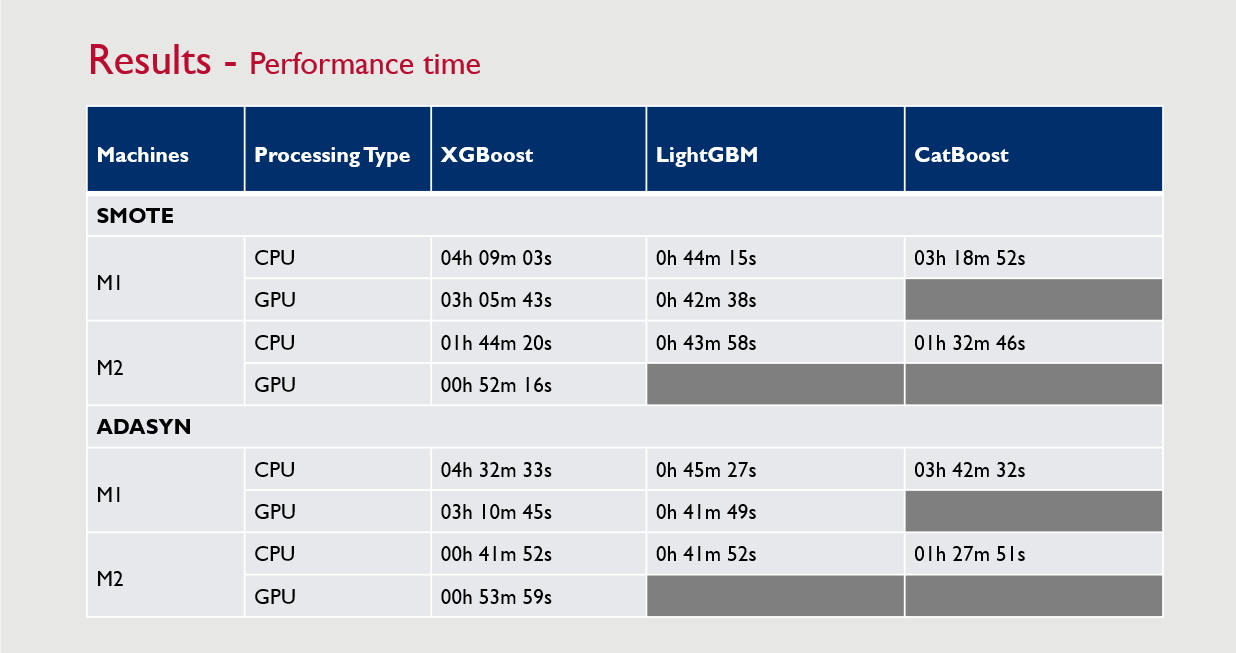
This data science project aimed to evaluate the performance of Gradient Boosting algorithms (XGBoost, LightGBM, and CatBoost) in predicting Home Credit Default Risk using balanced data. The study focused on improving predictive accuracy by addressing class imbalance, employing feature engineering, and optimizing model selection through resampling techniques (SMOTE and ADASYN).
The study followed a predictive analytics approach, leveraging machine learning models to forecast whether a customer will default on a loan. The models were assessed based on AUC, F1-score, training time, and inference time to determine the most effective algorithm for credit risk modeling.
The research was published as a scientific paper, contributing insights into credit risk prediction and the impact of class balancing on model performance.
✅ Predictive Analytics – Used machine learning models to predict credit default risk.
✅ Diagnostic Analytics – Assessed how class imbalance and resampling techniques impact model performance.
✅ Prescriptive Analytics – Recommended the most effective algorithm and resampling method based on performance evaluation.
The study utilized Home Credit Default Risk dataset, containing:
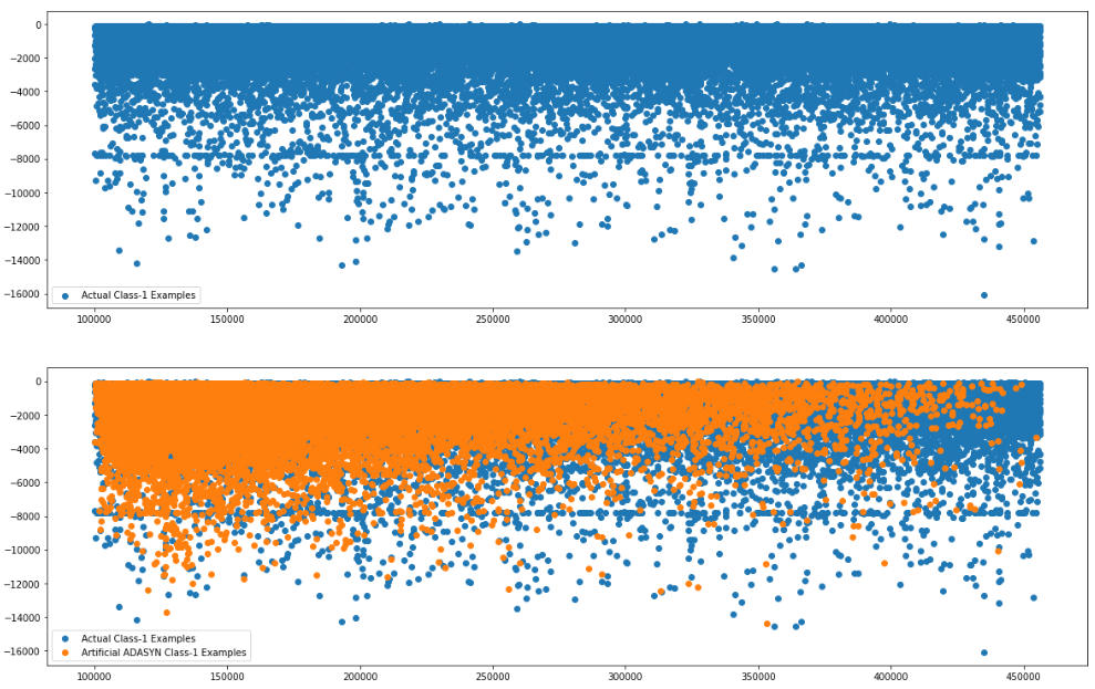
Since the dataset was highly imbalanced (more non-defaulters than defaulters), two oversampling techniques were used:
✔ SMOTE (Synthetic Minority Over-sampling Technique)
✔ ADASYN (Adaptive Synthetic Sampling)
This ensured an equal proportion of defaulters and non-defaulters, reducing bias in model predictions.
Trained and compared three Gradient Boosting models:
✔ XGBoost
✔ LightGBM
✔ CatBoost
Each model was evaluated on:
✔ ROC-AUC Score
✔ F1-Score
✔ Training Time
✔ Inference Time
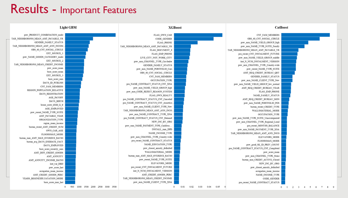
✔ Feature Importance
|
|
|
|
|
|
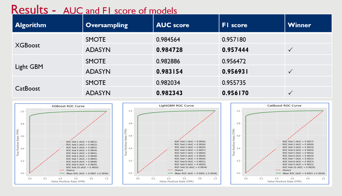
✔ XGBoost outperformed LightGBM and CatBoost in both AUC and F1-score.
✔ LightGBM was the fastest model in training and inference time.
✔ ADASYN performed better than SMOTE in improving model performance.
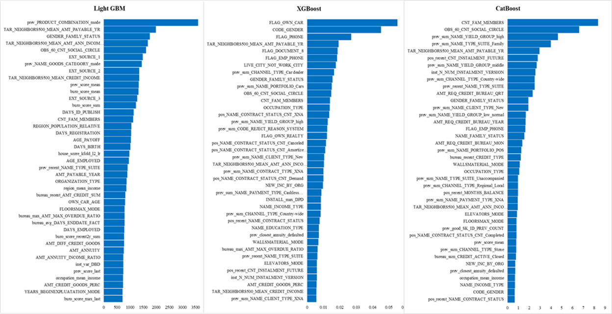
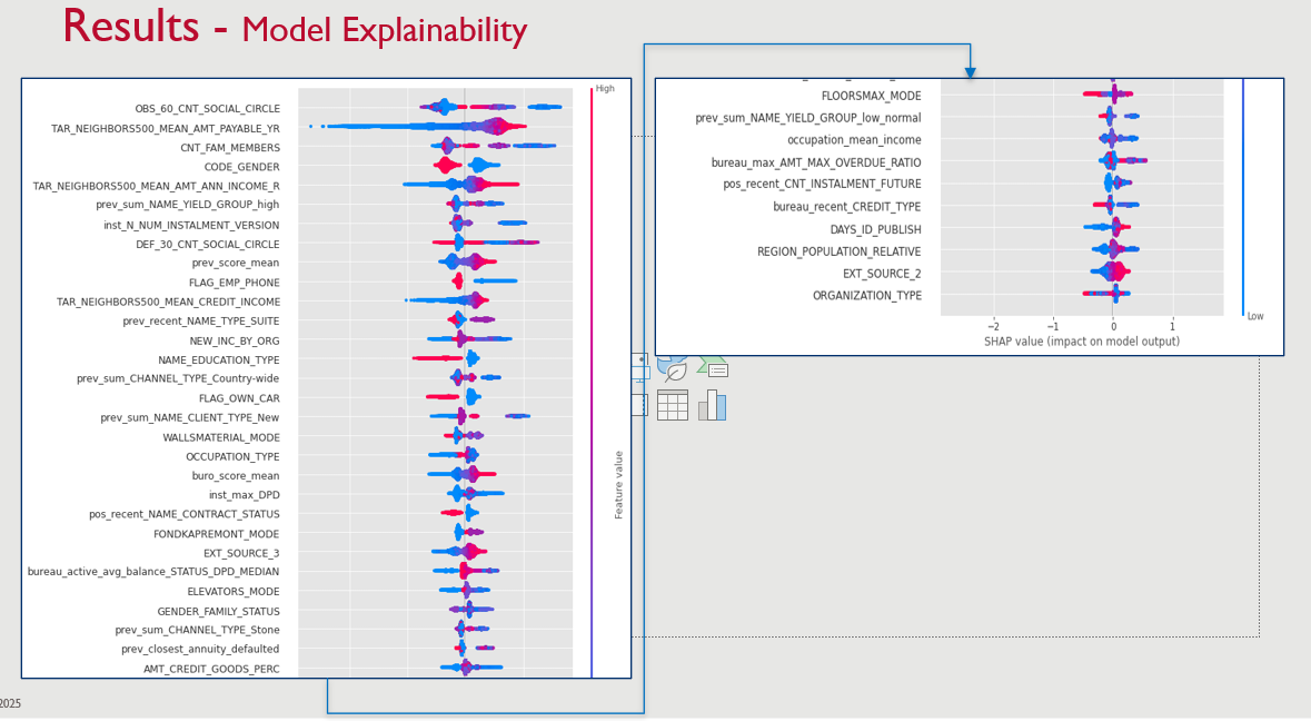
✔ All models provided feature importance insights, but key features differed across models.
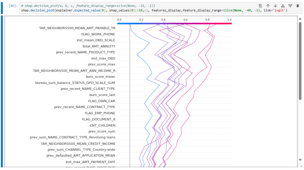
✔ SHAP values were used for model explainability, particularly for LightGBM.
✅ Challenge: High class imbalance → Solution: Applied SMOTE and ADASYN.
✅ Challenge: Large number of missing values → Solution: Multiple imputation methods (KNN, Iterative, Mean).
✅ Challenge: Computational efficiency → Solution: Optimized hyperparameters and used GPU acceleration for training.
To enhance interpretability, SHAP values were used to analyze:
Provided UNICEF, MoPH, implementers, and provincial health managers with a clear and comprehensive view of nutrition service expenditures and performance.
Enabled stakeholders to make data-driven decisions by highlighting key spending areas, donation allocations, and program effectiveness.
Automated ETL processes and data refreshes reduced manual effort and minimized errors, ensuring timely and accurate reporting.
Implemented Row-Level Security (RLS) to enable data access per user role without additional licensing costs, optimizing the project budget.
Embedded PowerBI dashboards into an ASP.NET Core application, enhancing accessibility and user satisfaction by providing a cohesive and user-friendly interface.
Delivered performance analysis metrics that allowed stakeholders to evaluate the effectiveness and efficiency of nutrition programs and expenditures.
Delivered a user-friendly interface and interactive dashboards that met the specific needs of UNICEF, MoPH, implementers, and provincial health managers.
Collaborated with UNICEF information specialist to define and implement critical metrics and KPIs, ensuring the dashboard meets user needs.
Consolidated data from SQL databases, SQL Server data, and APIs from approximately eight different sources to create a unified and comprehensive dataset.
Designed a scalable SQL Server data warehouse capable of handling large volumes of nutrition and health service data.
Developed robust ETL workflows using SSIS and Python to clean, transform, and integrate data from diverse sources.
Implemented an on-premises data gateway to automate data refreshes, ensuring the dashboard always displays the latest information.
Developed performance metrics and visualizations using DAX to evaluate the efficiency and effectiveness of nutrition programs and expenditures.
Performed comprehensive data modeling and wrote DAX formulas to create dynamic and insightful metrics for advanced data analysis.
✔ A study comparing three Gradient Boosting algorithms for Home Credit Default Risk Prediction.
✔ Provided empirical evidence that XGBoost performs best in AUC and F1-score, while LightGBM is the fastest.
✔ Showed that ADASYN is a better oversampling technique than SMOTE for improving performance.
✔ Identified key financial and demographic factors influencing credit default prediction.
✔ Published research that can be used by financial institutions to enhance risk assessment strategies.
The Evaluation of Gradient Boosting Algorithms on Balanced Home Credit Default Risk project showcases my ability to:
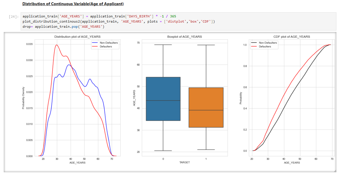
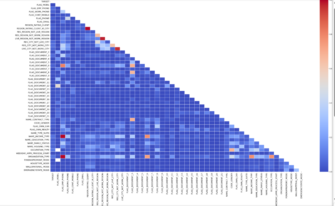
✔ Conduct Exploratory Data Analysis (EDA) to uncover key patterns.
✔ Perform Feature Engineering & Selection to improve model accuracy.
✔ Address Class Imbalance Issues with Resampling Techniques.
✔ Train & Evaluate Gradient Boosting Models to determine the best-performing algorithm.
✔ Use SHAP Values for Model Interpretability.
✔ Publish Research Findings that contribute to Financial Risk Prediction.
#FILTERING REQUIRED FEATURES
cate_features_name=['NAME_CONTRACT_TYPE', 'CODE_GENDER', 'FLAG_OWN_CAR', 'FLAG_OWN_REALTY', 'NAME_TYPE_SUITE',
'NAME_INCOME_TYPE', 'NAME_EDUCATION_TYPE', 'NAME_FAMILY_STATUS', 'NAME_HOUSING_TYPE', 'FONDKAPREMONT_MODE', 'HOUSETYPE_MODE',
'WALLSMATERIAL_MODE', 'EMERGENCYSTATE_MODE', 'GENDER_FAMILY_STATUS', 'bureau_CREDIT_ACTIVE_mode',
'pos_recent_NAME_CONTRACT_STATUS', 'prev_recent_NAME_CONTRACT_TYPE', 'prev_recent_NAME_CONTRACT_STATUS',
'prev_recent_NAME_PAYMENT_TYPE', 'prev_recent_CODE_REJECT_REASON', 'prev_recent_NAME_TYPE_SUITE',
'prev_recent_NAME_CLIENT_TYPE', 'prev_recent_NAME_PORTFOLIO', 'prev_recent_NAME_PRODUCT_TYPE', 'prev_recent_CHANNEL_TYPE',
'prev_recent_NAME_SELLER_INDUSTRY', 'prev_recent_NAME_YIELD_GROUP', 'prev_NAME_CONTRACT_TYPE_mode',
'prev_NAME_CASH_LOAN_PURPOSE_mode', 'prev_NAME_CONTRACT_STATUS_mode', 'prev_NAME_PAYMENT_TYPE_mode',
'prev_CODE_REJECT_REASON_mode', 'prev_NAME_TYPE_SUITE_mode', 'prev_NAME_CLIENT_TYPE_mode', 'prev_NAME_GOODS_CATEGORY_mode',
'prev_NAME_PORTFOLIO_mode', 'prev_NAME_PRODUCT_TYPE_mode',
'prev_CHANNEL_TYPE_mode', 'prev_NAME_SELLER_INDUSTRY_mode', 'prev_NAME_YIELD_GROUP_mode', 'prev_PRODUCT_COMBINATION_mode']
X_train[cate_features_name]=X_train[cate_features_name].astype("int32")
X_train = X_train.replace([np.inf, -np.inf], 0)
X_train=X_train.fillna(0)
X_train[cate_features_name].nunique()
#Balancing data using ADASYN
import warnings
warnings.filterwarnings("ignore")
from imblearn import over_sampling
ada = over_sampling.ADASYN(random_state=1000)
X_train_adasyn, y_train_adasyn = ada.fit_resample(X_train, y_train)
#----- Google colab because the column heading is missing due to Python version conflict-----
X_train_adasyn = pd.DataFrame(data=X_train_adasyn, columns=X_train.columns)
# Artificial minority samples and corresponding minority labels from ADASYN are appended
# below X_train and y_train respectively
# So to exclusively get the artificial minority samples from ADASYN, we do
X_train_adasyn_1 = X_train_adasyn[X_train.shape[0]:]
X_train_1 = X_train.to_numpy()[np.where(y_train==1.0)]
X_train_0 = X_train.to_numpy()[np.where(y_train==0.0)]
import matplotlib.pyplot as plt
%matplotlib inline
plt.rcParams['figure.figsize'] = [20, 20]
fig = plt.figure()
plt.subplot(3, 1, 1)
plt.scatter(X_train_1[:, 0], X_train_1[:, 1], label='Actual Class-1 Examples')
plt.legend()
plt.subplot(3, 1, 2)
plt.scatter(X_train_1[:, 0], X_train_1[:, 1], label='Actual Class-1 Examples')
plt.scatter(X_train_adasyn_1.iloc[:X_train_1.shape[0], 0], X_train_adasyn_1.iloc[:X_train_1.shape[0], 1],
label='Artificial ADASYN Class-1 Examples')
plt.legend()
plt.subplot(3, 1, 3)
plt.scatter(X_train_1[:, 0], X_train_1[:, 1], label='Actual Class-1 Examples')
plt.scatter(X_train_0[:X_train_1.shape[0], 0], X_train_0[:X_train_1.shape[0], 1], label='Actual Class-0 Examples')
plt.legend()
#FUNCTION TO CALCULATE OR FIND IMPORTANCE FEATURES
def feature_importances(feature_importance_df):
cols = feature_importance_df[["feature", "importance"]].groupby("feature").mean().sort_values(by="importance", ascending=False)[:50].index
best_features = feature_importance_df.loc[feature_importance_df.feature.isin(cols)]
plt.figure(figsize=(8, 12))
ticks=cols
ax=sns.barplot(x="importance", y="feature", data=best_features.sort_values(by="importance", ascending=False),color='gray')
plt.title('XGBoost Feature Importance')
r = ax.set_yticklabels(ticks, ha = 'left')
plt.draw() # this is needed because get_window_extent needs a renderer to work
yax = ax.get_yaxis()
# find the maximum width of the label on the major ticks
pad = max(T.label.get_window_extent().width for T in yax.majorTicks)
for tick_label in ax.axes.get_yticklabels():
tick_label.set_color("black")
yax.set_tick_params(pad=pad)
plt.tight_layout()
plt.show()
# FINDING BEST SCORERS
cate_features_name=ftures
import math
from sklearn.metrics import precision_recall_fscore_support
from sklearn.metrics import confusion_matrix ,classification_report
train_df = X_train_adasyn
y_train=y_train_adasyn
metrics_df = pd.DataFrame()
test_df = test.drop(columns=['TARGET'])
print("Starting XGBoost. Train shape: {}, test shape: {}".format(train_df.shape, test_df.shape))
folds = KFold(n_splits = 10, shuffle = True, random_state = 1001)
oof_preds = np.zeros(train_df.shape[0])
sub_preds = np.zeros(test_df.shape[0])
feature_importance_df = pd.DataFrame()
feats = [f for f in train_df.columns if f not in ['TARGET', 'SK_ID_CURR', 'SK_ID_BUREAU', 'SK_ID_PREV', 'index']]
start = datetime.now()
print('Start time: ', start)
for n_fold, (train_idx, valid_idx) in enumerate(folds.split(train_df[feats], y_train)):
train_x, train_y = train_df[feats].iloc[train_idx], y_train.iloc[train_idx]
valid_x, valid_y = train_df[feats].iloc[valid_idx], y_train.iloc[valid_idx]
clf = XGBClassifier(
n_jobs = -1,
n_estimators=3400,
tree_method = "hist",
colsample_bytree=0.4973019,
subsample=0.8129048,
learning_rate= 0.01,
max_depth=10,
reg_alpha=0,
reg_lambda=1,
# min_split_gain=0.0222415,
min_child_weight=5,
random_state = n_fold * 550
)
clf.fit(train_x, train_y, eval_set = [(train_x, train_y), (valid_x, valid_y)],
eval_metric = 'auc', verbose = True, early_stopping_rounds = 300)
# num_iteration=clf.classes_
oof_preds[valid_idx] = clf.predict_proba(valid_x )[:, 1]
sub_preds += clf.predict_proba(test_df[feats])[:, 1] / folds.n_splits
fold_importance_df = pd.DataFrame()
fold_importance_df["feature"] = feats
#https://eli5.readthedocs.io/en/latest/libraries/lightgbm.html
# weight = split
# https://stackoverflow.com/questions/37627923/how-to-get-feature-importance-in-xgboost
fold_importance_df["importance"] = clf.feature_importances_
fold_importance_df["fold"] = n_fold + 1
feature_importance_df = pd.concat([feature_importance_df, fold_importance_df], axis=0)
print('Fold %2d AUC : %.6f' % (n_fold + 1, roc_auc_score(valid_y, oof_preds[valid_idx])))
precision, recall, fscore, support = precision_recall_fscore_support(valid_y, oof_preds[valid_idx].round(),average='binary')
print('Fold %2d F1 Score binary : %.6f' % (n_fold + 1, fscore))
precision, recall, fscore2, support = precision_recall_fscore_support(valid_y, oof_preds[valid_idx].round(),average='macro')
print('Fold %2d F1 Score macro : %.6f' % (n_fold + 1, fscore2))
fpr, tpr, thresholds = roc_curve(valid_y, oof_preds[valid_idx])
fpr=np.mean(fpr)
tpr=np.mean(tpr)
# calculate the g-mean for each threshold
gmeans = math.sqrt(tpr * (1-fpr))
print('Fold %2d G-Mean of FPR and TPR : %.6f' % (n_fold + 1, gmeans))
getmetrics = {
'fold' : n_fold + 1,
'AUC Score' :roc_auc_score(valid_y, oof_preds[valid_idx]),
'F1 Score-binary' : fscore,
'F1 Score-macro':fscore2,
'G-Mean Score':gmeans,
'Type':'Fold Score',
"Model":"Model 1"
}
fold_metrics_df = pd.DataFrame(getmetrics, columns=['fold', 'AUC Score','F1 Score-binary','F1 Score-macro','G-Mean Score','Model'],index=[n_fold + 1])
metrics_df=pd.concat([metrics_df, fold_metrics_df], axis=0)
# End of modeling running
end = datetime.now()
total_time = end - start
print('Start time: ', start)
print('End time: ', end)
print('total timee: ', end - start)
xgboost_smote_time_df = pd.DataFrame({"Model":'Model 1',
"Start Time":start,
"End Time":end,
"Total Time":total_time}, index=[1])
# oof_preds=np.where(oof_preds<0.5,0,1)
print('Full AUC score %.6f' % roc_auc_score(y_train, oof_preds))
precision, recall, fscore, support = precision_recall_fscore_support(y_train, oof_preds.round(),average='macro')
print('Full F1 Score %.6f' % fscore)
gmeans = math.sqrt(tpr * (1-fpr))
print('Full G-Mean Score %.6f' % gmeans)
metrics_f= pd.DataFrame({"fold":6,
"AUC Score":roc_auc_score(y_train, oof_preds),
"F1 Score-binary":fscore,
"F1 Score-macro":fscore,
"G-Mean Score":gmeans,
"Type":"Full Score",
"Model":"Model 1"}, index=[6])
metrics_df=metrics_df.append(metrics_f)
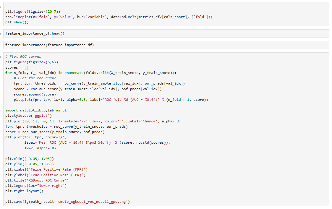
#PLOTTING AU AND F1 SCORE
cols_chart=['fold','AUC Score','F1 Score-macro']
metrics_df2=metrics_df[metrics_df['Model']=='Model 1']
plt.figure(figsize=(20,7))
sns.lineplot(x='fold', y='value', hue='variable', data=pd.melt(metrics_df2[cols_chart], ['fold']))
plt.show();
# Plot ROC curves
plt.figure(figsize=(6,6))
scores = []
plt.style.use('ggplot')
for n_fold, (_, val_idx) in enumerate(folds.split(y_train_adasyn, y_train_adasyn)):
# Plot the roc curve
fpr, tpr, thresholds = roc_curve(y_train_adasyn.iloc[val_idx], oof_preds[val_idx])
score = roc_auc_score(y_train_adasyn.iloc[val_idx], oof_preds[val_idx])
scores.append(score)
plt.plot(fpr, tpr, lw=1, alpha=0.3, label='ROC fold %d (AUC = %0.4f)' % (n_fold + 1, score))
plt.plot([0, 1], [0, 1], linestyle='--', lw=2, color='r', label='Chance', alpha=.8)
fpr, tpr, thresholds = roc_curve(y_train_adasyn, oof_preds)
score = roc_auc_score(y_train_adasyn, oof_preds)
plt.plot(fpr, tpr, color='g',
label='Mean ROC (AUC = %0.4f $\pm$ %0.4f)' % (score, np.std(scores)),
lw=2, alpha=.8)
plt.xlim([-0.05, 1.05])
plt.ylim([-0.05, 1.05])
plt.xlabel('False Positive Rate (FPR)')
plt.ylabel('True Positive Rate (TPR)')
plt.title('XGBoost ROC Curve')
plt.legend(loc="lower right")
plt.tight_layout()
# plt.savefig(path_result+'adasyn_lgbm_roc_model1_cpu.png')